Incident Field Types
ParticleScattering solves the multiple-scattering equation in the cylindrical wave domain, and thus a transformation is necessary in order to solve for arbitrary incident fields. The following field types are currently supported:
Plane Wave
A TM plane wave with angle $\theta_i$ relative to the x-axis is represented by
and constructed by calling PlaneWave(θ_i).
Line Current
Following standard notation, this is a line current with total current $I = i/k \eta$. This source cannot be placed inside a particle, and is constructed with LineSource(x0, y0).
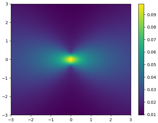
Current Source
A straight line containing an arbitrary single potential density \sigma, producing the following incident field:
The current density of this source is $J_z = i \sigma /k \eta$. Current sources must lie completely outside all particles, and are contructed with CurrentSource(x1, y1, x2, y2, σ), where (x1,y1) and (x2,y2) denote the start and end points, and σ is an array containing the single layer potential density at equidistant points along the source. For example,
using ParticleScattering, PyPlot
λ = 1
yc = range(-0.5λ, stop=0.5λ, length=100)
ui = CurrentSource(0, -0.5λ, 0, 0.5λ, cos.(π*yc/λ))
#now plot
x_points = 100; y_points = 100
x = range(-3λ, stop=3λ, length=x_points + 1)
y = range(-3λ, stop=3λ, length=y_points + 1)
xgrid = repeat(transpose(x), y_points + 1)
ygrid = repeat(y, 1, x_points + 1)
points = cat(2, vec(xgrid[1:y_points, 1:x_points]) + 3λ/x_points,
            vec(ygrid[1:y_points, 1:x_points]) + 3λ/y_points)
u = uinc(2π/λ, points, ui)
pcolormesh(xgrid, ygrid, abs.(reshape(u, y_points, x_points)))
colorbar()
yields the figure