Tutorial 2: Accelerating Solutions with FMM
In this tutorial, we examine scattering from several hundreds of particles, and use the built-in Fast Multipole Method (FMM) implementation to provide faster results. FMM groups nearby particles and approximates their cumulative effect on "far" particles. Here, the grouping is done by drawing a square grid over computational region encompassing the particles. The error of these approximations is fairly controllable, especially for mid- to high-frequency scattering.
Another difference between the direct and FMM solvers is that the latter requires an iterative solver for the system of equations (GMRES is used here). Thus a certain residual tolerance must be defined at which point the GMRES process terminates.
The scattering problem here is set up by
using ParticleScattering, PyPlot
λ0 = 1 #doesn't matter since everything is normalized to λ0
k0 = 2π/λ0
kin = 3k0
θ_i = π/4 #incident wave e^{i k_0 (1/sqrt{2},1/sqrt{2}) \cdot \mathbf{r}}

N_squircle = 200
N_star = 210
P = 10

M = 20
shapes = [rounded_star(0.1λ0, 0.03λ0, 5, N_star);
            squircle(0.15λ0, N_squircle)]
centers =  square_grid(M, λ0) #MxM grid with distance λ0
ids = rand(1:2, M^2)
φs = 2π*rand(M^2) #random rotation angles
sp = ScatteringProblem(shapes, ids, centers, φs)
To setup FMM, we use the constructor FMMoptions with the following options:
FMM::Bool       # Is FMM used? (default: false)
nx::Integer     # number of groups in x direction (required if dx is not
                # specified)
dx::Real        # group height & width (required if nx is not specified)
acc::Integer    # accuracy digits for translation truncation, and also for
                # GMRES if tol is not given (required)
tol::Real       # GMRES tolerance (default: 10^{-acc})
method::String  # method used: for now only "pre" (default: "pre")
For this problem, we choose $6$ digits of accuracy and grouping into $(M/2)^2$ boxes. The grouping can be viewed by calling divideSpace:
fmm_options = FMMoptions(true, acc = 6, nx = div(M,2))
divideSpace(centers, fmm_options; drawGroups = true)
In this plot, the red markers denote the group centers while stars denote particle centers (the particles can be drawn on top of this plot with draw_shapes). At first, it might look strange that parts of many particles lie outside the FMM group; however, the FMM is used only after the particles are converted to line sources, and are thus fully contained in the FMM grid.

Calculating and plotting the near or far fields with FMM is just as in the previous tutorial, except we must supply the FMMoptions object. We can also speed up the plotting by using the method = "recurrence" option:
plot_near_field(k0, kin, P, sp, PlaneWave(θ_i), opt = fmm_options,
    border = [-12;12;-10;10], x_points = 480, y_points = 400, method = "recurrence")
colorbar()

Note: Currently, FMM is used to accelerate the solution of the scattering problem, but not the field calculation in plot_near_field.
Direct vs. FMM timing
Which is more accurate?
Intuitively, the direct approach is more accurate than the FMM with its various approximations and iterative solution method. However, inaccuracies can arise in the direct solution of even the simplest scattering problems:
k0 = 0.01
kin = 0.02
shapes = [squircle(1, 200)]
ids = ones(Int, 64)
centers = square_grid(8, 5)
phis = zeros(64)
sp = ScatteringProblem(shapes, ids, centers, phis)
Pmax = 15
We solve this problem using the direct approach and with FMM, and then compare both the multipole coefficients $\beta$ and the resulting potential densities:
betas = Array{Vector}(undef, Pmax)
betas_FMM = Array{Vector}(undef, Pmax)
inners = Array{Vector}(undef, Pmax)
inners_FMM = Array{Vector}(undef, Pmax)
fmmopts = ParticleScattering.FMMoptions(true, nx = 4, acc = 9)
for P = 1:Pmax
	betas[P], inners[P] = solve_particle_scattering(k0, kin, P, sp, PlaneWave();
                            verbose = false)
	res, inners_FMM[P] = solve_particle_scattering_FMM(k0, kin, P, sp, PlaneWave(),
                            fmmopts; verbose = false)
	betas_FMM[P] = res[1]
end
import LinearAlgebra.norm
errnorm(x,y) = norm(x-y)/norm(x)

figure()
subplot(2,1,1)
semilogy(1:Pmax, [errnorm(betas_FMM[i], betas[i]) for i = 1:Pmax])
xlim([1;Pmax]); grid()
ylabel("\$\\Delta \\beta\$")
subplot(2,1,2)
semilogy(1:Pmax, [errnorm(inners_FMM[i], inners[i]) for i = 1:Pmax])
xlabel("\$ P \$")
xlim([1;Pmax]); grid()
ylabel("\$ \\Delta \$" * " Potential Density")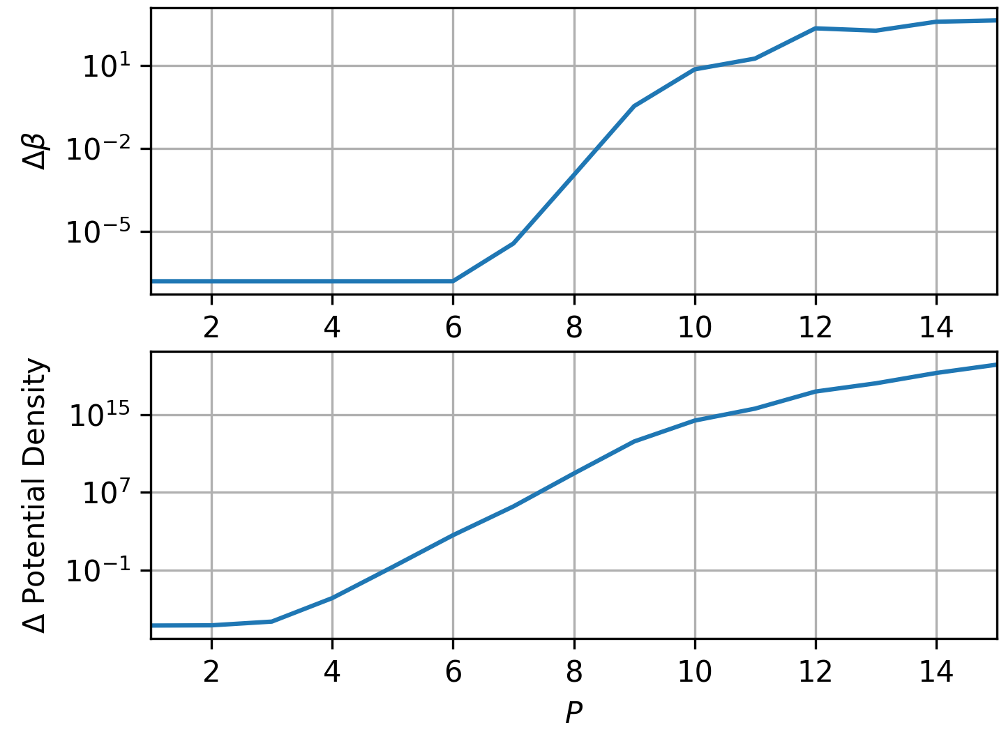
In both subplots, we see that increasing P actually leads to a decrease in accuracy (plotting the results separately also shows that the FMM results stay virtually constant, while the direct results blow up). This is due to two main reasons – conditioning of the system matrix, and the fact that high-order cylindrical harmonics are responsible for substantially greater potential densities than lower-order ones. Both of these are impacted by the number of particles as well as the wavelength, but mitigated by the iterative solver used by the FMM solver.
This ties in with Choosing Minimal N and P – not only does increasing P far beyond that required for a certain error impact runtime, but can also increase the error in the solution.