Tutorial 3: Angle Optimization

In this tutorial, we build upon the previous tutorial by optimizing the rotation angles of the particles (φs) to maximize the field intensity at a specific point. Depending on the scattering problem, wavelengths, and incident field, optimization can have a major or minor impact on the field. The simplest way to perform this optimization is by calling optimize_φ, which in turn utilizes Optim, a Julia package for nonlinear optimization. The type of objective function handled here is given by

where $I$ is a set of points that lie outside all scattering discs and $u$ is the $z$-component of the electric field. This function can be minimized directly, or maximized by minimizing $-f_{\mathrm{obj}}$.

First we set up our scattering problem:

λ0 = 1 #doesn't matter since everything is normalized to λ0
k0 = 2π/λ0
kin = 0.5k0
θ_i = 0 #incident wave e^{i k_0 (1/sqrt{2},1/sqrt{2}) \cdot \mathbf{r}}
pw = PlaneWave(θ_i)
M = 20
shapes = [rounded_star(0.35λ0, 0.1λ0, 4, 202)]
P = 12
centers =  rect_grid(2, div(M,2), λ0, λ0) #2xM/2 grid
ids = ones(Int, M)
φs0 = zeros(M)
sp = ScatteringProblem(shapes, ids, centers, φs0)
fmm_options = FMMoptions(true, acc = 6, dx = 2λ0)
points = 0.05*λ0*[-1 0; 1 0; 0 1; 0 -1]

where φs0 is the starting point for the optimization method, and points are the locations at which we intend to maximize or minimize the field intensity. In this case, we want to optimize intensity at a small area around the origin. We now select the optimization method and select its options. In most cases, BFGS with the default linesearch will yield accurate results in fast time; optimizing with adjoint = false requires a backtracking linesearch to reduce gradient evaluations. The possible convergence criteria are set by the bounds f_tol, g_tol, and x_tol, for a relative change in the function, gradient norm, or variables, respectively. In addition, we can set a maximum number of iterations. Verbosity of the output is set with show_trace and extended_trace.

import Optim
optim_options = Optim.Options(f_tol = 1e-6, iterations = 100,
                    store_trace = true, show_trace = true)
optim_method = Optim.BFGS()

We now run both minimization and maximization:

res_min = optimize_φ(φs0, points, P, pw, k0, kin, shapes, centers, ids,
            fmm_options, optim_options, optim_method; minimize = true)
res_max = optimize_φ(φs0, points, P, pw, k0, kin, shapes, centers, ids,
            fmm_options, optim_options, optim_method; minimize = false)
sp_min = ScatteringProblem(shapes, ids, centers, res_min.minimizer)
sp_max = ScatteringProblem(shapes, ids, centers, res_max.minimizer)

Once the optimization is done, we can visualize each ScatteringProblem separately with plot_near_field or compare them side by side with the following PyPlot code:

border = find_border(sp, points)
plts = Array{Any}(undef, 3)
for (i,spi) in enumerate([sp;sp_min;sp_max])
    global plts[i] = plot_near_field(k0, kin, P, spi, pw, x_points = 100,
                        y_points = 300, opt = fmm_options, border = border)
end

using PyPlot
fig, axs = subplots(ncols=3, figsize=[4.5,4])
for (i, spi) in enumerate([sp;sp_min;sp_max])
    global msh = axs[i].pcolormesh(plts[i][2][1], plts[i][2][2], abs.(plts[i][2][3]),
                        vmin = 0, vmax = 3.4, cmap="viridis")
    draw_shapes(spi, ax = axs[i])
    axs[i].set_aspect("equal", adjustable = "box")
    axs[i].set_xlim([border[1];border[2]])
    axs[i].set_ylim([border[3];border[4]])
    axs[i].set_xticks([-1,0,1])
    i > 1 && axs[i].set_yticks([])
    axs[i].set_xlabel("x")
end
axs[1].set_ylabel("y")
subplots_adjust(left=0.12, right=0.8, top=0.98, bottom = 0.12, wspace = 0.1)
cbar_ax = fig.add_axes([0.83, 0.12, 0.05, 0.86])
fig.colorbar(msh, cax=cbar_ax)
cbar_ax.set_ylabel("|E\$_z\$ [V/m]")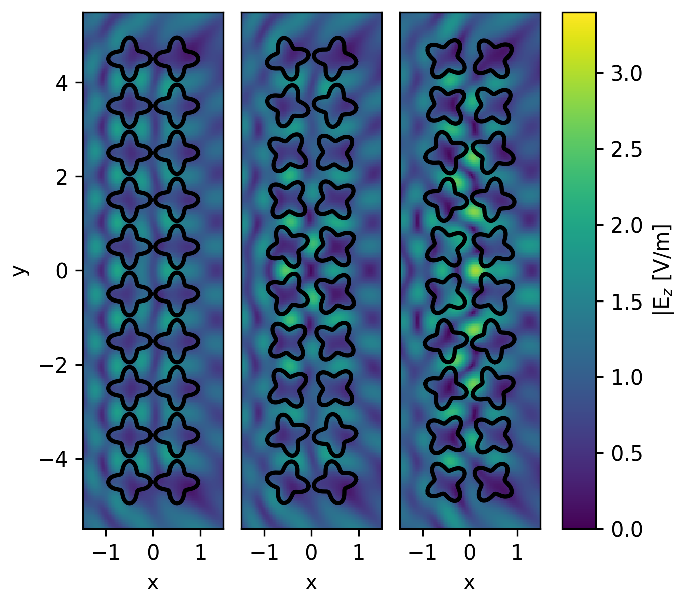

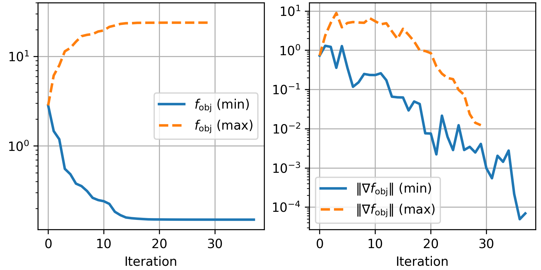
From left to right, we see the electric field before optimization, after minimization, and after maximization. The field intensity at the origin is notably different in both optimization results, with minimization decreasing the intensity at points by 77%, and maximization almost tripling it. The convergence of the optimization method for both examples can be plotted via:

iters = length(res_min.trace)
fobj = [res_min.trace[i].value for i=1:iters]
gobj = [res_min.trace[i].g_norm for i=1:iters]
iters2 = length(res_max.trace)
fobj2 = -[res_max.trace[i].value for i=1:iters2]
gobj2 = [res_max.trace[i].g_norm for i=1:iters2]

fig, axs = subplots(ncols=2, figsize=[6,3])
axs[1].semilogy(0:iters-1, fobj, linewidth=2)
axs[2].semilogy(0:iters-1, gobj, linewidth=2)
axs[1].semilogy(0:iters2-1, fobj2, linewidth=2, "--")
axs[2].semilogy(0:iters2-1, gobj2, linewidth=2, "--")
axs[1].legend(["\$f_\\mathrm{obj}\$ (min)";
                "\$f_\\mathrm{obj}\$ (max)"], loc="right")
axs[2].legend(["\$\\Vert \\nabla f_\\mathrm{obj}\\Vert\$ (min)";
                "\$\\Vert \\nabla f_\\mathrm{obj}\\Vert\$ (max)"], loc="best")
axs[1].set_xlabel("Iteration")
axs[2].set_xlabel("Iteration")
axs[1].set_ylim(ymax=40)
axs[1].grid(); axs[2].grid()
subplots_adjust(top=0.99, right=0.99, left=0.07, bottom=0.15)