Tutorial 4: Radius Optimization

In this tutorial, we explore radius optimization, whereby the radii of a group of circular particles are optimized simultaneously to minimize or maximize the electric field intensity at a group of points.

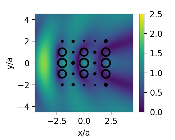
We begin by defining a standard scattering scenario with a $5 \times 5$ square grid of particles:

using PyPlot, ParticleScattering
import Optim

er = 4.5
k0 = 2π
kin = sqrt(er)*k0
a = 0.2*2π/k0     #wavelength/5
θ_i = 0.0
pw = PlaneWave(θ_i)
P = 5
centers = square_grid(5, a)
φs = zeros(size(centers,1))
fmm_options = FMMoptions(true, acc = 6, dx = 2a)

optimize_radius not only allows us to optimize all of the radii simultaneously, but also to assign several particles the same id, which can be useful when the target radii are expected to have symmetry of some type. Here we shall assume symmetry with respect to the $x$-axis with uniqueind:

# let's impose symmetry wrt x-axis
centers_abs = centers[:,1] + 1im*abs.(centers[:,2])
ids, centers_abs = uniqueind(centers_abs)
J = maximum(ids) #number of optim vars

The same could be done for the $y$-axis, both axes simultaneously, or radial symmetry, by appropriately choosing center_abs. We now define the optimization parameters via Optim.Options, with convergence decided by the radii and a limited number of 5 outer iterations (with up to 5 inner iterations each). We choose to minimize the field intensity at a single point outside the structure, assert that this point will remain outside the particles regardless of their size, and set the lower and upper bounds for each circle:

optim_options =  Optim.Options(x_tol = 1e-6, outer_x_tol = 1e-6,
                               iterations = 5, outer_iterations = 5,
                               store_trace = true, show_trace = true,
                               allow_f_increases = true)

points = [4a 0.0]
r_max = (0.4*a)*ones(J)
r_min = (1e-3*a)*ones(J)
rs0 = (0.25*a)*ones(J)
@assert verify_min_distance(CircleParams.(r_max), centers, ids, points)

The optimization process is initiated by running:

res = optimize_radius(rs0, r_min, r_max, points, ids, P, pw, k0, kin,
                centers, fmm_options, optim_options, minimize = true)
rs = res.minimizer

With the optimization process complete, we can plot the electric field with the initial and optimized radii:

sp1 = ScatteringProblem(CircleParams.(rs0), ids, centers, φs)
plot_near_field(k0, kin, P, sp1, pw, x_points = 150, y_points = 150,
        opt = fmm_options, border = 0.9*[-1;1;-1;1], normalize = a)
colorbar()
clim([0;2.5])
xlabel("x/a")
ylabel("y/a")
sp2 = ScatteringProblem(CircleParams.(rs), ids, centers, φs)
plot_near_field(k0, kin, P, sp2, pw, x_points = 150, y_points = 150,
        opt = fmm_options, border = 0.9*[-1;1;-1;1], normalize = a)
colorbar()
clim([0;2.5])
xlabel("x/a")
ylabel("y/a")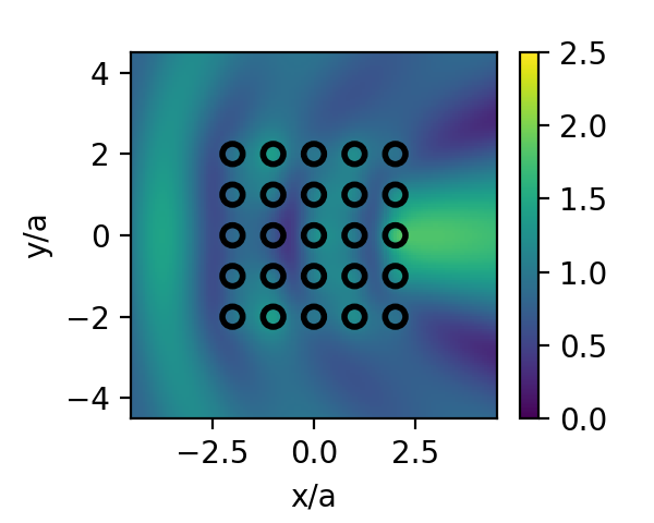

res also stores the objective value as well as the g radient norm in each iteration. This can be extracted by

inner_iters = length(res.trace)
iters = [res.trace[i].iteration for i=1:inner_iters]
fobj = [res.trace[i].value for i=1:inner_iters]
gobj = [res.trace[i].g_norm for i=1:inner_iters]
rng = iters .== 0

where rng now contains the indices at which a new outer iteration has begun. Finally, plotting fobj and gobj for this example yields the following plot:

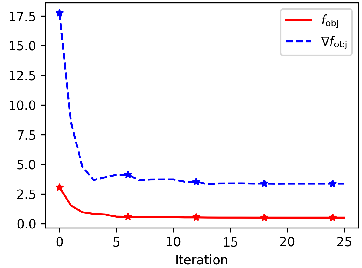
where markers denote the start of an outer iteration.